TempEst-NEXT Real-Time National Forecasting

import NEXT
import NEXT.wforecast as wfc
import os
import matplotlib.pyplot as plt
import pandas as pd
import geopandas as gpd
import shapely as shp
from pynhd import WaterData, NLDI
from time import sleep
import warnings
import numpy as np
import datetime

Prepare Environment

dirs = ["hist_data/", "hrrr_data/", "final_hist/", "gfs_raw/", "forecasts/", 'figures/', 'full_forecasts/']
for d in dirs:
    if not os.path.exists(d):
        os.mkdir(d)

Identify Sites

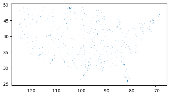
By default, the forecast runs for 1,000 HUC-12 pour points sampled from across the contiguous US. You can modify this by changing the site selection below and removing the cached site file. The sampling procedure is to select 1,000 different HUC-8s, then sample one HUC-12 from each. (The actual default dataset contains 913 sites after misc errors.)

sitefile = "forecast_points.json"
run_sites = not os.path.exists(sitefile)

def try_and_sleep(f):
    sleep(5)
    try:
        return f()
    except:
        return None

# Wait between calls because otherwise it tends to overload the API
if run_sites:
    huc6 = WaterData("wbd06")
    huc12 = WaterData("wbd12")
    all_huc6 = huc6.bybox((-125, 25, -65, 50))
    huc12_samp = pd.concat([
        try_and_sleep(lambda: huc12.bygeom(x.geometry).sample(n=50)) # get extra samples because some will crash
        for x in all_huc6.itertuples()
    ]).sample(n=1200)
    pps = NLDI().getfeature_byid("huc12pp", huc12_samp["huc12"])
    geodata = (huc12_samp.loc[:, ["geometry", "huc12", "areasqkm"]].
        rename(columns={"huc12": "id", "areasqkm": "area"}).
        merge(
            pd.DataFrame({
                "id": pps["identifier"],
                "lat": pps.geometry.y,
                "lon": pps.geometry.x
            }),
            on="id"
        )).dropna().sample(1000)
    geodata.loc[:, "area"] = geodata["area"] * 1e6 # km2 -> m2
    geodata.to_file(sitefile)

else:
    geodata = gpd.read_file(sitefile)

geodata.plot()

<Axes: >

Retrieve Historical Data

Humidity is retrieved from GridMet. Air temperature is from HRRR so that climatology will be more similar to GFS, for which NEXT doesn’t have long-term archive retrieval (just recent forecast runs).

The below loops may crash periodically due to server errors. If so, just restart them, as they are set up to resume where they left off. GridMet retrieval takes several hours, and HRRR retrieval is currently exceptionally slow for no obvious reason, on the order of 1 hour per site. Due to that challenge, HRRR is only retrieved for one year for a sample of sites, which is used to fit a correction function.

runhist = len(os.listdir(dirs[2])) == 0

basepath = dirs[0] + "/"
if runhist:
    with warnings.catch_warnings(action="ignore"):
        for row in geodata.itertuples():
            fn = basepath + row.id + ".csv"
            if not os.path.exists(fn):
                # note: site type "huc12" doesn't actually exist. It will internally convert to coordinates.
                try:
                    NEXT.data.geom_full_data(row.id, "huc12", gpd.GeoSeries([row.geometry], crs=4326), row.lat, row.lon, row.area,
                                             "2015", "2025", "gridmet").to_csv(fn, index=False)
                except:
                    print(row.id)

The following block can be cancelled after several dozen sites have been retrieved.

if runhist:
    allids = [x.split('.')[0] for x in os.listdir(dirs[0])]  # don't run HRRR if we don't have other info
    basepath = dirs[1] + '/'
    with warnings.catch_warnings(action="ignore"):
        for row in geodata.itertuples():
            fn = basepath + row.id + ".csv"
            if (not os.path.exists(fn)) and (row.id in allids):
                NEXT.data.weather_hrrr(gpd.GeoSeries([row.geometry], crs=4326), "2025-01-01", "2025-12-31").to_csv(fn, index=False)

Compute corrections:

allids = [x.split('.')[0] for x in os.listdir(dirs[1])]
combined = pd.concat([
    pd.read_csv(dirs[0] + "/" + row.id + ".csv", parse_dates=["date"]).
        merge(pd.read_csv(dirs[1] + "/" + row.id + ".csv", parse_dates=["date"]),
              on="date",
              suffixes=["_gm", "_hrrr"])
    for row in geodata.itertuples()
    if row.id in allids
])

combined.plot.scatter(x="tmax_gm", y="tmax_hrrr")

<Axes: xlabel='tmax_gm', ylabel='tmax_hrrr'>

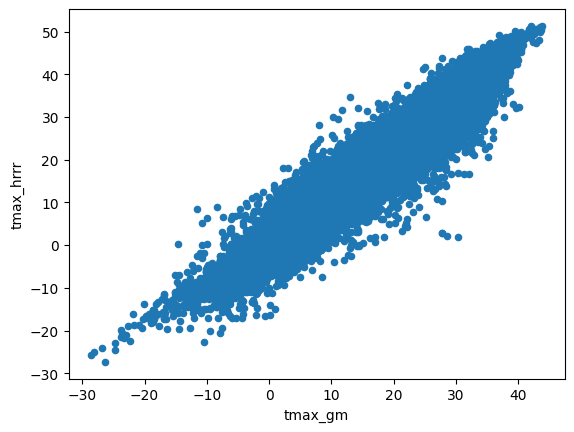
combined["tmax_gm"].corr(combined["tmax_hrrr"])

np.float64(0.9543465835168514)

(combined.groupby("id")[["tmax_hrrr", "tmax_gm"]].corr().
    loc[(slice(None), "tmax_gm"), "tmax_hrrr"].describe())

count    78.000000
mean      0.945189
std       0.037704
min       0.762891
25%       0.935038
50%       0.956855
75%       0.967331
max       0.978917
Name: tmax_hrrr, dtype: float64

The relationship is imperfect, but we observe that sitewise correlation is nearly identical to global correlation, so a global correction can be applied.

fit = np.linalg.lstsq(
    np.array([np.ones(len(combined)), combined["tmax_gm"]]).T,
    combined["tmax_hrrr"])[0]

if runhist:
    for fn in os.listdir(dirs[0]):
        if fn.endswith('.csv'):
            data = pd.read_csv(dirs[0] + "/" + fn, parse_dates=["date"])
            data["tmax"] = data["tmax"] * fit[1] + fit[0]
            data.to_csv(dirs[2] + '/' + fn, index=False)

Retrieve Forecast Data and Execute Forecasts

model = NEXT.NEXT.from_pickle('coefs_hrrr.pickle')

allids = [x.split('.')[0] for x in os.listdir(dirs[2])]
torun = geodata.loc[geodata['id'].isin(allids)]
earlier = (datetime.date.today() - datetime.timedelta(6)).strftime("%Y%m%d")
today = datetime.date.today().strftime("%Y%m%d")
with warnings.catch_warnings(action='ignore'):
    fcst_weath = (pd.concat([wfc.get_gfs_downloaded(torun, earlier, dirs[3]),
                             wfc.get_gfs_downloaded(torun, today, dirs[3])]).
        groupby(["id", "date"], as_index=False)["tmax"].last().sort_values("date"))
    for row in torun.itertuples():
        infn = dirs[2] + row.id + '.csv'
        outfn = dirs[4] + row.id + '_' + today + '.csv'
        if not os.path.exists(outfn):
            try:
                model.make_newt(pd.read_csv(infn, parse_dates=['date']), reset=True)
                model.run(fcst_weath.loc[fcst_weath['id'] == row.id]).to_csv(outfn, index=False)
            except KeyboardInterrupt:
                break
            except:
                print(row.id)

080901000101

Analyze The Forecast

today = datetime.date.today().strftime("%Y%m%d")
forecast = pd.concat([
    pd.read_csv(dirs[4] + fn, parse_dates=['date']).
        assign(id = fn.split('_')[0])
    for fn in os.listdir(dirs[4])
    if today in fn and fn.endswith('.csv')
])
# Limit to weekly forecast
forecast = forecast.loc[(forecast['date'] >= np.datetime64('today')) &
    (forecast['date'] < np.datetime64('today') + 7)]
forecast = forecast.merge(geodata, on='id').dropna()
forecast.drop(columns=['day', 'period', 'geometry']).to_csv(dirs[6] + today + '.csv', index=False)
forecast

	id	date	tmax	day	period	prediction	seasonal	anomaly	area	lat	lon	geometry
0	010900050201	2026-04-13	15.362663	103	103	8.945897	10.911749	-1.965852	66570000.0	41.442098	-71.590871	MULTIPOLYGON (((-71.51761 41.55376, -71.51733 ...
1	010900050201	2026-04-14	21.079019	104	104	9.638248	11.044416	-1.406168	66570000.0	41.442098	-71.590871	MULTIPOLYGON (((-71.51761 41.55376, -71.51733 ...
2	010900050201	2026-04-15	23.610065	105	105	10.816572	11.177676	-0.361104	66570000.0	41.442098	-71.590871	MULTIPOLYGON (((-71.51761 41.55376, -71.51733 ...
3	010900050201	2026-04-16	21.855503	106	106	11.754032	11.311491	0.442541	66570000.0	41.442098	-71.590871	MULTIPOLYGON (((-71.51761 41.55376, -71.51733 ...
4	010900050201	2026-04-17	23.611570	107	107	11.973921	11.445821	0.528099	66570000.0	41.442098	-71.590871	MULTIPOLYGON (((-71.51761 41.55376, -71.51733 ...
...	...	...	...	...	...	...	...	...	...	...	...	...
6449	030601020108	2026-04-15	28.654725	105	105	9.599104	9.068038	0.531067	68530000.0	34.716343	-83.354611	MULTIPOLYGON (((-83.39605 34.78676, -83.39639 ...
6450	030601020108	2026-04-16	27.555318	106	106	11.424976	8.912083	2.512893	68530000.0	34.716343	-83.354611	MULTIPOLYGON (((-83.39605 34.78676, -83.39639 ...
6451	030601020108	2026-04-17	29.583026	107	107	11.641974	8.755528	2.886446	68530000.0	34.716343	-83.354611	MULTIPOLYGON (((-83.39605 34.78676, -83.39639 ...
6452	030601020108	2026-04-18	28.607069	108	108	11.782561	8.598419	3.184142	68530000.0	34.716343	-83.354611	MULTIPOLYGON (((-83.39605 34.78676, -83.39639 ...
6453	030601020108	2026-04-19	24.017823	109	109	10.909466	8.440803	2.468663	68530000.0	34.716343	-83.354611	MULTIPOLYGON (((-83.39605 34.78676, -83.39639 ...

6454 rows × 12 columns

# Export to mappable GeoJSON. Modify this code to set custom color scales. These column
# labels work with CalTopo.
fcjs = forecast.groupby(['lat', 'lon', 'id'])['prediction'].agg(['mean', 'min', 'max'])
fcjs = gpd.GeoDataFrame(fcjs,
                        geometry = [
                            shp.Point(x.lon, x.lat)
                            for x in fcjs.reset_index().itertuples()
                        ],
                        crs=4326)
fcjs['marker-size'] = 2
fcjs['title'] = fcjs.index.get_level_values('id')
fcjs['marker-color'] = "0000FF"
fcjs.loc[fcjs['mean'] > 10, 'marker-color'] = "008080"
fcjs.loc[fcjs['mean'] > 13, 'marker-color'] = "00FF00"
fcjs.loc[fcjs['mean'] > 16, 'marker-color'] = "808000"
fcjs.loc[fcjs['mean'] > 20, 'marker-color'] = "FF0000"
fcjs.to_file(dirs[6] + today + '_map.json')

Forecast Description

Warning: this is an experimental stream water temperature forecast for the upcoming week. Results are not guaranteed in any capacity. Typical errors are approximately 2.5 C (4 F); any given prediction may have considerably higher errors. For example, in the southern Rocky Mountains during the first forecast run (April 2026), the model, while it did predict high temperature anomalies, was unable to fully account for the unseasonal loss of snowpack and therefore underpredicted temperatures by several degrees.

These data and related items of information have not been formally disseminated by NOAA, and do not represent any agency determination, view, or policy. This research is funded by the NOAA Cooperative Institute for Research to Operations in Hydrology.

The code used to generate these forecasts is available on GitHub at https://github.com/mines-ciroh/natl-temp-forecast (requires support for ecCodes, for which Linux is recommended). Additionally, required preliminary data for the 913 default forecast sites are available on the GitHub Releases page, so the only data retrieval required is the GFS forecast download. Actual weekly forecasts are made available on CUAHSI HydroShare at http://www.hydroshare.org/resource/b8852529788a437a8d697e9b0435b99a.

The US states shapefile was retrieved from https://www.census.gov/geographies/mapping-files/time-series/geo/carto-boundary-file.html, and the large rivers shapefile from https://www.weather.gov/gis/Rivers. Both were converted to GeoJSON.

forecast[['seasonal', 'anomaly', 'prediction']].describe()

	seasonal	anomaly	prediction
count	6454.000000	6454.000000	6454.000000
mean	12.242600	0.017864	12.260464
std	6.945637	1.836547	6.939229
min	-9.059694	-8.743582	0.000000
25%	7.109645	-0.788977	7.080628
50%	11.700867	0.149350	12.294008
75%	18.104874	1.022540	18.170668
max	33.877230	9.553768	34.791661

states = gpd.read_file("states.json")
states = states.loc[~states["STUSPS"].isin(["AK", "HI", "PR"])]  # CONUS
rivers = gpd.read_file("rivers.json")

def signed_max_abs(series):
    # Find the largest absolute value, preserving sign
    mx = series.max()
    mn = series.min()
    if abs(mx) >= abs(mn):
        return mx
    return mn
def scale_size(series, mn=1, mx=5, ceiling=5):
    series = series.abs()
    series.loc[series > ceiling] = ceiling
    return mn + (series - series.min()) * (mx - mn) / (series.max() - series.min())

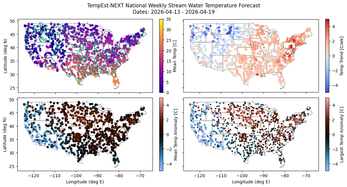
fig, axes = plt.subplots(2, 2, sharex=True, sharey=True, figsize=(12, 6), layout='compressed')
for axr in axes:
    for ax in axr:
        states.plot(facecolor="none", edgecolor="#606060", ax=ax, linewidth=0.8, linestyle='dashed')
(forecast.groupby('id')[['lat', 'lon', 'prediction']].mean().
    rename(columns={'prediction': 'Mean Temp [C]'}).
    plot.scatter(
    x='lon', y='lat', c='Mean Temp [C]',
        cmap='plasma', vmin=0, vmax=35, ax=axes[0, 0],
    ylabel='Latitude (deg N)', xlabel='Longitude (deg E)'))
rivers.loc[rivers["STRAHLER"] > 3].plot(ax=axes[0, 0], linewidth=1, edgecolor='teal')
(forecast.groupby('id').agg({'lat': 'mean', 'lon': 'mean', 'anomaly': 'mean'}).
    rename(columns={'anomaly': 'Mean Temp Anomaly [C]'}).
    plot.scatter(
    x='lon', y='lat', c='Mean Temp Anomaly [C]',
        cmap='berlin', vmin=-5, vmax=5, ax=axes[1, 0],
    ylabel='Latitude (deg N)', xlabel='Longitude (deg E)'))
(forecast.groupby('id').agg({'lat': 'mean', 'lon': 'mean', 'anomaly': signed_max_abs}).
    assign(anomsize=lambda x: scale_size(x['anomaly'], mn=3, mx=20)).
    rename(columns={'anomaly': 'Largest Temp Anomaly [C]'}).
    plot.scatter(
    x='lon', y='lat', c='Largest Temp Anomaly [C]', s='anomsize',
        cmap='berlin', vmin=-5, vmax=5, ax=axes[1, 1],
    ylabel='Latitude (deg N)', xlabel='Longitude (deg E)'))
# Compute weekly *trend*
start = forecast.loc[forecast['date'] == forecast['date'].min()].set_index('id')
end = forecast.loc[forecast['date'] == forecast['date'].max()].set_index('id')
start.loc[:, 'Temp Trend [C/wk]'] = end['prediction'] - start['prediction']
start.plot.scatter(x='lon', y='lat', c='Temp Trend [C/wk]',
        cmap='coolwarm', vmin=-5, vmax=5, ax=axes[0, 1],
    ylabel='Latitude (deg N)', xlabel='Longitude (deg E)')
fig.suptitle(f'''TempEst-NEXT National Weekly Stream Water Temperature Forecast
Dates: {forecast['date'].min().date()} - {forecast['date'].max().date()}''')
fig.savefig(dirs[5] + f'ForecastPlot_{today}.png', dpi=300)